climate-weather/ai produced the result/ · v2
Benchmarking the cost of ensemble Kalman methods for calibrating chaotic models
Researchers measured how much computation four ensemble Kalman calibration methods need to recover known parameters of chaotic toy climate models. In one test, the quantity being fitted was the 61 weights of a small neural network standing in for an unresolved forcing.
spectrum · one line per step, placed by what the step does · bright lines used AI
The Ensemble Kalman Inversion Race
doi:10.1029/2025ms005629 · record aix-00306 v2 · checked 2026-11-16
- AI was for
- Simulation surrogate
- Model family
- Multilayer perceptron, Gaussian process
- Checked by
- Held-out100 tested
- Code
- available
The finding the paper is about came from the AI.
What this research was about
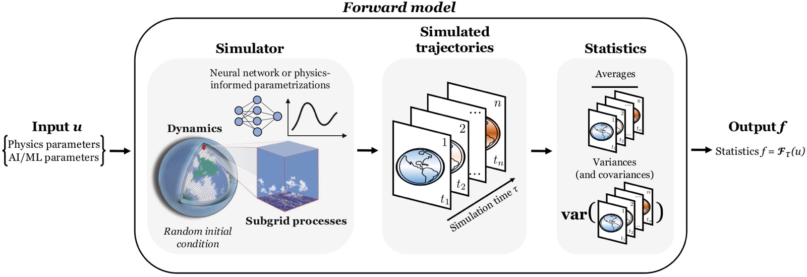
Climate models contain settings that cannot be measured directly, such as how strongly small-scale processes push the large-scale flow. These settings have to be tuned until the model's long-run statistics match observations. That tuning is awkward for two reasons. The systems are chaotic, so two runs from almost identical starting points diverge, and only time-averaged quantities such as means and variances are stable enough to compare. And each trial run is expensive, so the number of model runs a tuning method needs is the quantity that matters. One family of methods, ensemble Kalman inversion, avoids needing derivatives of the model by running a spread of parameter guesses at once and updating them towards the data.
The researchers set up a race between four such methods, labelled TEKI, ETKI, UKI and IEKF, on small chaotic test systems (the Lorenz '63 and Lorenz '96 models) where the true parameters were known in advance. Synthetic data were time-averaged statistics of the simulated state, with observation error estimated from windowed longer runs. Each method was run until it reached a stated accuracy, at the ensemble size that minimised the number of model runs, averaged over 100 randomised repetitions. A derivative-based optimiser, Levenberg-Marquardt, was run on the same problems for comparison; the authors report that it did not reach the target accuracies in any test problem.
Where AI came in
Neural networks appear here as the thing being fitted rather than as a tool for prediction. In one test problem, the forcing that varies across the Lorenz '96 grid was represented by a shallow neural network: one input (the position on the grid), one output (the local forcing) and 20 internal units, giving 61 weights and biases. Those 61 numbers were the unknowns, and the ensemble Kalman methods estimated them from time-averaged statistics of the simulated state. The network therefore stands in for a hand-written formula for a process the model does not resolve, turning a modelling choice into a calibration problem with many more unknowns than a handful of physical constants.
Networks were also fitted beforehand to set up starting assumptions, the prior. For a vague prior, smooth candidate forcing functions were drawn from a Gaussian process (a standard way of sampling random smooth curves) and a network was trained on each draw; the resulting spread of weights fixed the prior's mean and covariance. For a more pointed prior, the mean came from a network fitted to a shifted and squashed version of the true forcing. A further fit to the sinusoidal forcing defined the 'true' weights. The authors report that UKI rarely reached the target accuracy under the vague neural network prior, while TEKI and ETKI reached it with both priors.
Written by AIxSci from the checked record below, to give context for readers outside the field. It is not part of the record.
The work
Technical · from the record
The study compares how much computation several ensemble Kalman methods (TEKI, ETKI, UKI and IEKF) need to estimate parameters of chaotic Lorenz-type models from noisy time-averaged statistics, a setting used as a stand-in for climate model calibration. One test problem replaces a spatially varying Lorenz '96 forcing with a shallow neural network of 20 neurons whose 61 weights and biases are estimated online by the ensemble methods, and neural networks are also fitted offline to construct informative and uninformative prior distributions. Each method is run to target accuracies of RMSE 1, 1.1 and 1.2 at an ensemble size chosen to minimise the number of forward model runs, with averages taken over 100 randomized repetitions. The authors report that no single method was cheapest in all test problems, that UKI needed the fewest forward runs when only one or two parameters were estimated but rarely reached the target RMSE under the uninformative neural network prior, that TEKI and ETKI reached the targets in the neural network problems with and without an informative prior, and that Levenberg-Marquardt did not reach the target RMSEs in any test problem.
How AI was used
Neural networks appear in two roles, both fitted within the study. In the Lorenz '96 test problem with a spatially varying forcing, a shallow network with a scalar input (the spatial index) and a scalar output (the local forcing) and 20 neurons is used as the forcing parameterization, and its 61 weights and biases are the unknowns estimated online by the ensemble Kalman methods from time-averaged statistics of the simulated state. Separately, networks are fitted offline to build prior distributions over those weights: for the uninformative prior, smooth functions are drawn from a periodic Gaussian process with a Gaussian kernel and length scale 8 and a network is trained on each draw, with the resulting weight sets defining the prior mean and covariance; for the informative prior, the mean is the weights of a network fitted to a randomly translated and compressed version of the true forcing, with a scaled identity covariance. A further offline fit to the sinusoidal forcing, trained on sampled input/output pairs, defines the 'true' weight values against which slices of the loss function are drawn. The ensemble Kalman iterations themselves, and the Levenberg-Marquardt baseline run through SciPy's least_squares wrapper around MINPACK, are derivative-free or derivative-based optimisation procedures rather than learned models. Forward models are fourth-order Runge-Kutta integrations of Lorenz '63 and Lorenz '96 systems, and observation error covariances are sample covariances of windowed statistics from longer simulations.
The shape of the work
Structural · the record, drawn
Simulate chaotic dynamics and generate synthetic statistical data
Numerical or physics simulation, including where a learned surrogate replaces it.
The forward model maps model parameters/parameterizations to statistical datawhere the paper describes this · verbatim
Estimate observation error covariance from windowed long simulations
Cleaning, filtering, normalising or labelling data already obtained.
we run a simulation of duration ns⋅τ and then window the simulation output to compute ns samples of statistical datawhere the paper describes this · verbatim
Fit neural networks offline to define true weights and prior distributions
Fitting model parameters, including fine-tuning an existing model.
and then train neural networks on each drawwhere the paper describes this · verbatim
Calibrate model parameters and neural network weights with ensemble Kalman methods
Fitting model parameters, including fine-tuning an existing model.
We apply various ensemble methods (TEKI, ETKI, UKI, IEKF) to estimate model parameters or parameterizations from time-averaged data.where the paper describes this · verbatim
Sweep ensemble sizes and select the optimal ensemble size
Iterative search over a space. Its result feeds back into an earlier step.
To determine the optimal ensemble size we solve the same problem for a range of ensemble sizeswhere the paper describes this · verbatim
Run derivative-based Levenberg-Marquardt baseline on the same problems
Iterative search over a space.
We use LM within Python and SciPy's least_squares algorithmwhere the paper describes this · verbatim
Compare recovered parameters and computational cost against the known truth
Testing outputs against ground truth.
We then measure the computational cost each ensemble method requires to find a solution with a specified accuracywhere the paper describes this · verbatim
What the record says
Technical · every part carries its own basis
+ in the paper~ our reading− not reported
How to read the quotations. A quotation shows where the paper describes something. It does not quote every value beside it: one passage locates a part of the work, and values without their own quotation are our reading of that passage.
The paper's result is a measured comparison of calibration algorithms; the runs that produce it include fitting the weights and biases of a neural network parameterization, and neural networks are also fitted offline to build priors. A reviewer could instead argue for 'analysis', since the neural network appears in only part of the test suite and the ensemble Kalman algorithms themselves are derivative-free inverse methods rather than learned models.
We use a shallow NN with 20 neurons and perform online learning to obtain the nu=61 weights and biases of the NN parameterization.where the paper describes this · verbatim
We address this issue by performing 100 experiments (at each ensemble size)where the paper describes this · verbatim
The software and synthetic data used to generate the results in this paper are uploaded to both Github and Zenodo.where the paper describes this · verbatim
What this paper did not report
Technical · absence is published deliberately
- Trained model weightsWhether the trained model is available is not stated.
- ComputeThe hardware or time used is not stated.
- What step 3 replacedThe paper gives no basis for what the AI stood in for.
- What step 4 replacedThe paper gives no basis for what the AI stood in for.
About this article
Record aix-00306, version 2, checked by a person on 2026-11-16. The record describes the paper; it does not assess whether the paper's findings are right. The paper is published under CC-BY; quotations are at most 25 words. How we work · Report an error
Cite this record: AIxSci (2026). Benchmarking the cost of ensemble Kalman methods for calibrating chaotic models. Record aix-00306, version 2, checked 2026-11-16. https://aixsci.org/articles/aix-00306/